


Abstract
Quantum entanglement lies at the heart of quantum mechanics in both fundamental and practical aspects. The entanglement of quantum states has been studied widely both theoretically and experimentally, however, the entanglement of operators has not been studied much experimentally in spite of its importance. Here, we propose a scheme to realize arbitrary entangled operations based on a coherent superposition of local operations with a non-zero probability of failure. Then, we experimentally implement several intriguing two-qubit entangled operations in photonic systems. We also discuss the generalization of our scheme to extend the number of superposed operations and the number of qubits. Due to the simplicity of our scheme, we believe that it can reduce the complexity or required resources of the quantum circuits and provide insights to investigate properties of entangled operations.
Export citation and abstract BibTeX RIS

Original content from this work may be used under the terms of the Creative Commons Attribution 4.0 licence. Any further distribution of this work must maintain attribution to the author(s) and the title of the work, journal citation and DOI.
1. Introduction
Entanglement is the key concept that makes quantum physics distinct from classical physics and plays an essential role in quantum information processing. As an entangled state cannot factor into a product of individual states, entangled operations cannot be represented by a product of individual operations but a coherent superposition of operations [1–5]. To date, superpositions of operators have been studied in both fundamental and practical aspects. Commutation relations for bosonic operators [6] and Pauli operators [7, 8] have been directly demonstrated experimentally using superpositions of operators, also Hamiltonian dynamics based on superposition of operations has been proposed theoretically [9]. Recently, it is reported that the superpositions of quantum operations can allow controlling the orders of quantum operations, which is not allowed in the traditional formalism of quantum physics [10–12]. This, so-called superposition of causal orders, is not only fundamentally interesting but also proven that it has practical applications in quantum information processing in the context of communication complexity [13, 14], witnessing causality [15, 16], quantum metrology [17], and transmission of quantum information [18].
However, so far research on superposition of quantum operations has been limited to superposition of single qubit gates in most cases, meaning that entanglement of operators has not been studied much yet. Most of the implementations of superposition of causal orders are relying on the interferometric scheme, however, in this case extension to an entangled operation is not straightforward since nonlocality should be involved. Extension to implementing an entangled operation is particularly important since a two-qubit entangled operation such as controlled-NOT (CNOT) gate can constitute the universal sets of quantum gates with single qubit gates [19–21]. Implementation of entangled operations for two-qubit systems can provide further advantages for practical quantum information processing, such as entanglement filter (EF) [22–24], entangling gate for universal quantum gate set [25], and entanglement generation for teleportation-based programmable quantum gate [7, 26–28]. It is also intriguing to explore entangled operations in even larger Hilbert spaces for investigating potential applications in quantum information processing.
In this letter, we propose and demonstrate a scheme for realizing an arbitrary entangled operation based on a coherent superposition of local operations. We first begin by introducing the concept of operator entanglement using an operator-Schmidt decomposition. We then present some intriguing and important operations that can be realized based on this scheme in two-qubit systems. Then, we describe our experimental demonstration of several two-qubit entangled operations in photonic systems and discuss our experimental results. Finally, we extend our scheme to the case of generalized entangled operations with N qubit systems and the Schmidt number M. We also present a practical scheme on implementing three-qubit entangled operations and introduce interesting three-qubit operations that can be implemented.
2. Theory
An operator  acting on systems A and B can be written as

where ci ⩾ 0 and  is orthonormal bases for a system A (B) [5]. Similar to the Schmidt representation of quantum states, equation (1) is the operator-Schmidt decomposition and the number of nonzero Schmidt coefficients ci is defined as a Schmidt number [5]. If the Schmidt number of an operator
  is larger than one,
  is an entangled operator meaning that it can generate entanglement from separable states. It is clear that
  with i = 1 could be prepared by local operations and classical communications between two distant systems A and B. However, in general, an operator having higher Schmidt number (i ⩾ 2) needs to implement a coherent superposition of operators
  with different i [5].
Let us consider a simple case with the Schmidt number 2 and c1 = c2. Then,

where  ,
,  ,
,  ,
,  and ϕ is the relative phase between A1 ⊗ B1 and A2 ⊗ B2. Note that the second line of equation (2) is not the Schmidt decomposition due to the complex number of coefficients, but it can explicitly show the relative phase ϕ between two superposed operations. In many cases, local operations are fixed but their relative phase can be varied. The entangled operation of equation (2) has a simple form, however, there are intriguing operations. When A1 = B1 = I, A2 = B2 = σx, equation (2) becomes

where I is an identity operation and σx, σy, and σz are Pauli operators. One can prepare maximally entangled states  (
( ) from a separable input state
  (
( ).
).
When  , B1 = I,
  , and B2 = U where U is a single qubit unitary operation, one can implement a controlled-unitary (CU) operation. In addition, by setting A1 = B1 = |0⟩⟨0|, A2 = B2 = |1⟩⟨1|, one can realize the EF which is a special non-unitary operation, and transmits the input states only when the incoming qubit states is either |0⟩|0⟩ or |1⟩|1⟩ [22–24].
However, it is difficult to implement an entangled operation of equation (2). Using an interferometer, it is possible to make a superposition of two different operators such as  [8]. However, when the system A and B use interferometers separately, what they prepare is
  , which has clearly the Schmidt number 1. Note that if we apply A1 and B1 simultaneously to the system A and B with the half of the time and apply A2 and B2 with another half of the time, the prepared operation is an incoherent mixture of A1 ⊗ B1 and A2 ⊗ B2 rather than a coherent superposition of them.
3. Experiment
Here, we propose a scheme for implementing an entangled operations using additional degree of freedom. The conceptual diagram of our scheme is shown in figure 1. For a two-qubit input state  , qubit an undergoes an operation A1 or A2 while qubit B undergoes an operation B1 or B2. In order to prepare an entangled operation, one needs to rule out A1 ⊗ B2 and A2 ⊗ B1 cases and the other two cases A1 ⊗ B1 and A2 ⊗ B2 should be coherently superposed. It is difficult to achieve these requirements, however, it is possible by using energy–time correlation of spontaneous parametric down conversion (SPDC) process. In experiment, the input state is encoded in a polarization of single photons. When a pair of photons are generated via SPDC process, the generated photon pairs have strong energy–time correlation. By exploiting this strong time correlation between two photons, one can prepare a coherent superposition of local operations, e.g.,
  acting on polarization states of two-photons.

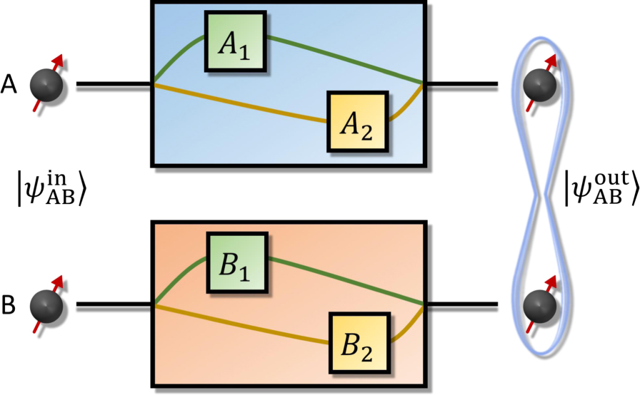
Figure 1. Concept of two-qubit entangled operation with the Schmidt number 2. Two-qubit input states  undergoes either operation A1 ⊗ B1 (green line) or A2 ⊗ B2 (orange line). Here, these two processes are coherently superposed so that the output state is
  . For a separable input state, the output state can be entangled. Note that the entangled operation can be implemented only with local operations if we use additional degree of freedom (ancillary systems).
Download figure:
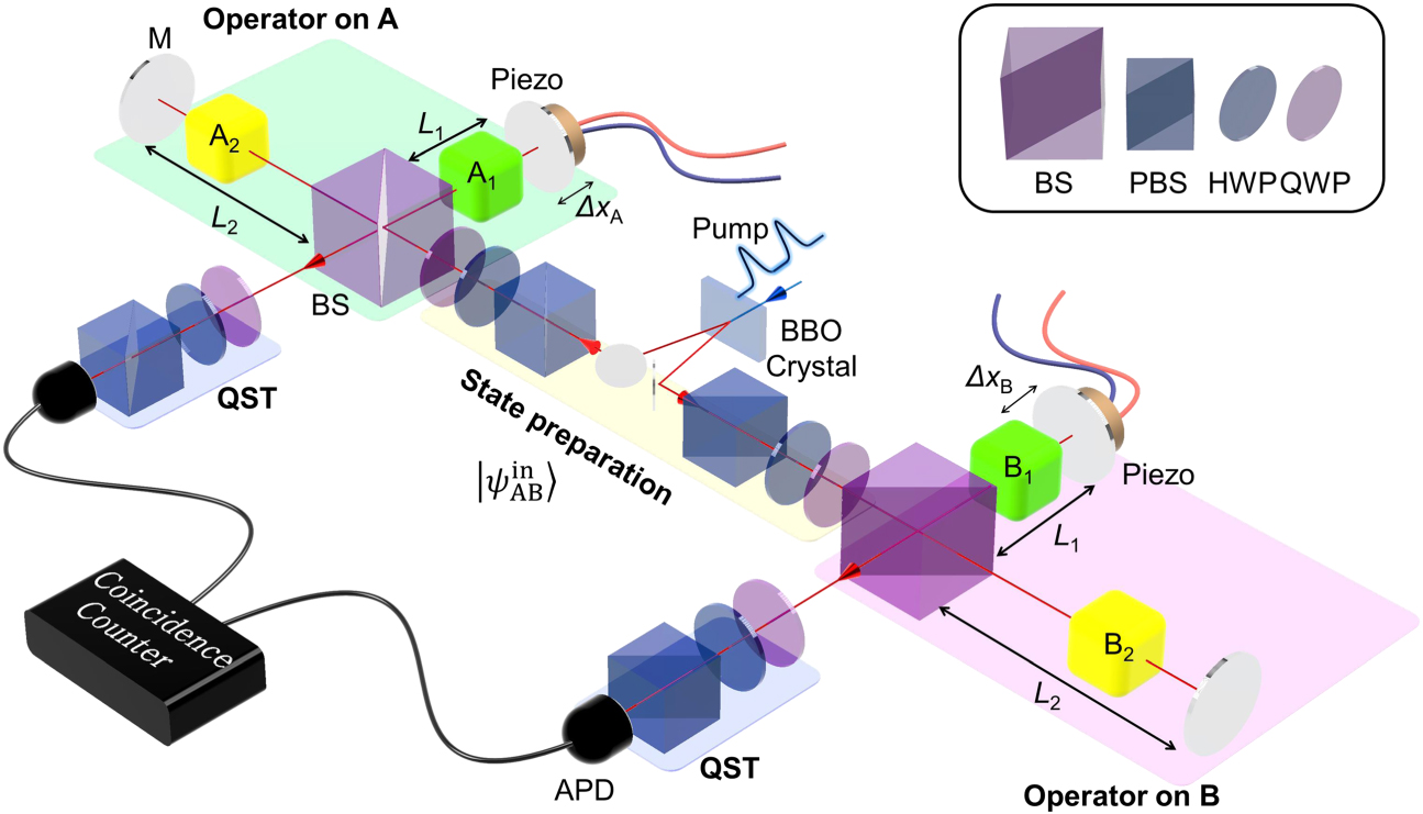
Standard image High-resolution imageThe schematic of our experimental setup is shown in figure 2, which is based on Franson interferometer [29, 30]. We use a femtosecond pulsed laser operating at a center wavelength of 780 nm and a pulse period of 12.5 ns. The wavelength of the pump laser becomes 390 nm using a lithium triborate (LBO) crystal via second harmonic generation (SHG) process. Then, a pair of photons is generated via type-II SPDC process by pumping a 1 mm-thick beta-barium borate (BBO) crystal, and its polarization state is prepared in an arbitrary input state  with a set of polarizer, half and quarter wave plates (WPs). Then, each photon is sent to an unbalanced Michelson interferometer (UMI) with different optical lengths of L1 and L2. The path length different L = L2 − L1 is 1.875 m corresponding to an half of the pulse period of the pump laser to ensure that the down-converted photons generated from consecutive pump pulses are temporally overlapped. Here we use an interference filter with 2 nm full-width at half maximum bandwidth, then the coherence length of each down-converted photon is around 300 μm. Hence, there is no first order interference at the output of UMI. In order to implement
  in equation (2), single qubit operations A1 and A2 (B1 and B2) are located in L1 and L2 arms of the UMI for a photon A (photon B), respectively. Note that a single qubit operation can be realized by linear optical elements such as WPs, polarizer (Pol.), and so on. The two-photon output states are analyzed by a set of WPs and Pol. using quantum state tomography (QST) and quantum process tomography (QPT).

Figure 2. Schematic of the experimental set-up. A down-converted photon pair generated from a pulsed laser is prepared in an arbitrary polarization two-photon state  using a set of Pol., HWP, and QWP. Single qubit operations (A1, A2, B1, and B2) can be realized with linear optical elements such as Pol. and WPs, and the relative phase between two arms of an UMI is controlled by adjusting ΔxA and ΔxB, respectively. Entangled operations are implemented with two UMIs. A set of Pol. and WPs in front of APD are used to perform QST measurements (BBO: beta barium borate crystal, QST: quantum state tomography, M: mirror, APD: avalanche photo diode, QWP: quarter waveplate, HWP: half waveplate, Pol.: polarizer, BS: beam splitter, PBS: polarizing beam splitter).
Download figure:
Standard image High-resolution imageLet us describe the process of entangled operations of  for input state
  as following transformations:

The system and ancilla qubits are encoded, respectively, on the polarization, |ψ⟩, and time-bin modes |t⟩. After implemented prepared operations with experimental set-up as shown in figure 2, there are four possible output cases as second step of equation (4). Here |t1⟩ and |t2⟩ refer to qubit arrived from short and long path of UMI, respectively. Then we can post-select output state as  . Here, we used a measurement operator as
  , which is implemented by set the coincidence window (we use 3 ns) smaller than the time difference between L1 and L2 (12.5 ns). Note that this is possible due to strong time correlation between temporally overlapped photon pairs using UMI which has path length difference corresponding to pulse period of photon pairs. Note that mixed states can be prepared by adjusting the path length difference L of UMI differently from an half of the pulse period of the pump laser, then it reduces the temporal overlap of the down-converted photons generated from consecutive pump laser pulses. The post-selected output state
  becomes
  where ϕ is the sum of relative phase differences in each UMI (ϕ = ϕA + ϕB). In order to fix ϕ, we attached piezoelectric actuators on both mirrors in the short arms of the UMI and drive them using proportional integral derivative (PID) controllers to lock the relative phases ϕA and ϕB. Here, we can choose ϕ between 0 to 2π using a set of QWP, HWP, and QWP on the locking laser (780 nm pump laser). See appendix
4. Results
We demonstrated various entangled operations based on our experimental setup shown in figure 2. The first entangled operation we consider is  with A1 = B1 = σz and A2 = B2 = σx, i.e.,
  .
.  is able to generate entanglement since for a separable input state
  , the output state is
  , the maximally entangled states. We implemented
  with ϕ = 0, π/2, π, and 3π/2 and performed QST measurement to each output states. The density matrices of the output states are reconstructed using maximum-likelihood method [31, 32] and the experimental results are shown in figure 3. As shown in figure 3, one can adjust the relative phase ϕ and the realized operation works well. Note that for the input state
  , the output state becomes
  . See appendix
  .
.

Figure 3. Reconstructed density matrices of the output state after the entangled operation  . Input state is prepared to |HH⟩, and σx and σz are implemented by using QWP with an angle of π/4 and 0, respectively. The expected output state after the entangled operation is
  . The reconstructed density matrices of the output states correspond to (a) ϕ = 0, (b) π/2, (c) π, and (d) 3π/2. Note that the upper (lower) rows corresponds to the real (imaginary) part of the density matrices. The average fidelity between the ideal output state and the experimentally obtained output state is Fave = 0.940 ± 0.014 and the average concurrence of the output states C = 0.906 ± 0.025. We performed Monte-Carlo simulations on reconstructing density matrices of each output state 100 times and the calculated experimental errors corresponds to one standard deviation.
Download figure:
Standard image High-resolution imageIn order to show the quality of the implemented operation, we also performed QPT measurement. Figure 4 shows the experimentally reconstructed process matrices χ for entangled operations  and
and  . The corresponding process fidelities Fχ are 0.760 ± 0.005 and 0.762 ± 0.006, respectively. Here we use
 ![${F}_{\chi }={\left[\mathrm{Tr}\left(\sqrt{\sqrt{{\chi }_{\mathrm{exp}}}{\chi }_{\text{ideal}}\sqrt{{\chi }_{\mathrm{exp}}}}\right)\right]}^{2}$](https://content.cld.iop.org/journals/1367-2630/22/9/093070/revision2/njpabb64aieqn45.gif) where χideal (χexp) is the process matrix of the ideal (experimentally realized) operation. Note that Fχ results are obtained by performing 100 Monte-Carlo simulations on the QPT measurement results and the errors on the process fidelities corresponds to one standard deviation. We also provide QPT results of
where χideal (χexp) is the process matrix of the ideal (experimentally realized) operation. Note that Fχ results are obtained by performing 100 Monte-Carlo simulations on the QPT measurement results and the errors on the process fidelities corresponds to one standard deviation. We also provide QPT results of  operation in appendix

Figure 4. Experimentally reconstructed process matrices χ of the entangled operations. (a).  . (b)
. (b)  . We reconstructed process matrices using maximum-likelihood method on QPT results. Left (right) columns corresponds to the real (imaginary) part of the process matrices. Process matrices are represented in the Pauli basis, for example, YZ corresponds to σy, σz basis.
Download figure:
Standard image High-resolution imageNote that in general, a coherent superposition of unitary operators is not a unitary operator. The operator  is composed of unitary operators but it is a non-unitary operator. On the other hand,
  is a unitary operation. It is known that if UAB is a two-qubit unitary operation with Schmidt number 2, UAB has the form of
  up to local unitary equivalence where 0 ⩽ p ⩽ 1 [5]. Hence, one can realize any two-qubit unitary operations with Schmidt number 2 using our scheme. Moreover, it is interesting to consider the possibility of emulating Ising gate, which is a two-qubit gate implemented natively in trapped-ion quantum system, based on our scheme [33, 34]. For example,
  is exactly the same with 3π/4 Ising (XX) gate [34]. Note that, Ising (XX) gate and single-qubit rotation gates can constitute a universal set of quantum gates.
5. Perspectives: generalization to M superposed operations  for N qubit

We emphasize that entangled operations can be extended to the case of M superposed operations  for N qubit states by adding optical arms of the interferometers and adding the number of interferometers, respectively, then
  is given by

where  is the kth local operation acting on jth qubit and ck is the Schmidt coefficient. Note that ck is adjustable using BS having different reflectivity and transmittivity ratio. Figure 5(a) shows an unbalanced Mach–Zehnder interferometer (UMZI) with four different arms. For an interferometer A, the local operation Ai with i = 0, 1, 2, 3 is located in each arm of the UMZI where the optical path length difference is fixed to L between two neighboring arms and it is the same for the interferometer B. Then, one can prepare an entangled operation with Schmit number 4 of

by post-selecting the case where the arrival time difference of two-photons is zero and ϕi with i = 1, 2, 3 is the relative phase differences. In this case, all the other terms are not detected [29, 30]. It is well-known that any two-qubit operation can be decomposed into the form of equation (6) up to local unitary equivalence [35]. Note that we can implement SWAP gate  based on the setup shown in figure 5(a). Considering the CNOT complexity of SWAP gate is three [36], i.e., three consecutive CNOT gates are required for a single SWAP gate, it significantly reduces the implementation complexity of SWAP gate.

Figure 5. Generalization to the entangled operation with higher Schmidt number and multipartite systems. (a) For two-qubit input states, one can increase the number of optical paths of the UMZI. Then, the entangled operation with higher Schmit number can be realized. (b) By adding one more UMZI, one can implement tripartite entangled operations.
Download figure:
Standard image High-resolution imageWe can also consider increasing the number of qubits by adding more UMZIs as shown in figure 5(b). For example, three photon input states can be prepared by using cascaded SPDC process [37]. In this case, we consider three qubit systems and the corresponding three qubit entangled operation  is
is

where  are single qubit operations acting on qubit C. For example, one can obtain three qubit Greenberger–Horne–Zeilinger state [38]
  from an input state
  by implementing
  . Likewise, if one implement
  , then one can prepare three qubit W state [39]
  from an input state
  . Moreover, one can implement the controlled–controlled-unitary (CCU) gate
  . If U = σx, then this operation becomes the Toffoli (controlled–controlled NOT) gate [40].
6. Summary
In summary, we have proposed a scheme to implement arbitrary entangled operations based on a coherent superposition of local operations. We also report an experimental demonstration of various two-qubit entangled operations in photonic systems. We believe that our scheme has great importance both in fundamental and practical aspects. Entanglement of operators is closely related to the evolution of quantum systems under nonlocal Hamiltonians and the entangling power of quantum operators [2, 3, 41]. In addition, it is known that superposition of quantum gates cannot be represented by the conventional quantum circuit models [42] and the extended quantum circuit model allowing such superposition of operators can reduce the computational complexity of some problems and simplify realization of various quantum information processing [11, 43]. Due to the simplicity of our scheme and the possibility to extend to multi-qubit systems, it is interesting to apply our scheme to solve practical problems using quantum algorithms such as Hamiltonian simulation [9] and quantum chemistry problem [44]. Moreover, although we mainly discuss unitary operations but the scheme can also be applicable to non-trace-preserving operations. Hence, it is intriguing to consider exploring PT symmetry broken operations [45] and adding a control to weak measurements or partial collapse measurement [46].
Acknowledgments
We acknowledge funding from KIST institutional program (Project No. 2E30620) and the National Research Foundation of Korea (Grant Nos. 2019M3E4A1079526).
Appendix A.: Experimental details
390 nm pulse train is prepared by 1 mm thick LBO crystal via SHG process using a 780 nm mode-locked pump laser (80 MHz repetition rate, 140 fs pulse duration, M2 < 1.1, Chameleon, Coherent), and generates photon pairs via type-II SPDC process at a 1 mm thick BBO crystal. The 780 nm pump laser is separated by a DM from 390 nm laser, and used as a locking laser to lock the relative phase between two arms of an UMI. The locking laser enters a one-inch cube BS spatially separated from the single photon's path in order not to be detected at APD. In order to actively lock the relative phase between two arms of UMI from mechanical and thermal vibrations of optical components, we implement a PID control system as shown in figure A1.

Figure A1. Experimental setup for implementing two-qubit entangled operation  . LBO: lithium triborate, DM: dichroic mirror, FBS: fiber beam splitter, BBO: beta-barium borate, BS: beam splitter, PBS: polarizing beam splitter, HWP: half wave plate, QWP: quarter wave plate, PID: proportional–integral–derivative, PD: photo detector, APD: avalanche photo diode, Att: attenuator.
Download figure:
Standard image High-resolution imageA.1. Locking the relative phase between two arms of an UMI
We test the performance of our phase locking system using a single balanced Michelson interferometer (MI), meaning that the path length difference between two arms is negligible. Single photon and locking laser are injected to a single balance MI, and the intensity of the locking laser is controlled by driving the voltage to a piezo actuator attached on the mirror of one arm. Then, we measure the single photon count of the signal (down-converted photons) using an APD depending on the intensity of the locking laser. As shown in figure A2(a), we can observe the interference fringes of both signal (black line) and locking laser (red line) at the same time by scanning the mirror on one arm using a piezo actuator (see figure A2(a) after 3600 s). Then, we fixed the intensity of the locking laser around the half of the maximum intensity of the interference fringe by using a PID controller and a voltage amplifier, which enables locking the relative phase between two arms of MI. As shown in figure A2(a), signal is locked to have the minimum count by adjusting the phase using α when intensity of the locking laser is half of the maximum intensity of interference fringe. Figure A2(b) shows the stability of phase locking in the interferometer during an hour, we find that the relative phase on signal is locked. We have considered that the imperfections of our experimental results (purity, concurrence, and fidelity) are mainly due to the phase fluctuation. We implement an entangled operation  using a single UMI instead of two UMIs and the results shows the better performance. We will compare this results at the section 3.

Figure A2. Results on active phase locking of an MI. The relative phase of an balanced MI is locked by fixing the intensity of locking laser to around the half of the maximum intensity, and we find that single photon signal is also locked simultaneously. Red (black) line corresponds to the intensity of the locking laser (single photon signals). (a) Correlation between the locking laser intensity and the single photon signal. They are locked at the same time during phase locking is on. We can observe that interference fringes of the locking laser and the signal simultaneously by applying a periodic voltage to the piezo actuator. (b) We monitor the intensity change of the locking laser and the signal during an hour while the locking system is on.
Download figure:
Standard image High-resolution imageIn order to control the relative phase ϕ of  from 0 to 2π in two UMIs, we use a set of QWP (π/4)–HWP (α)–QWP (π/4) for locking laser on the long arm of the UMI on qubit A, see figure A1. This waveplate combination provides the phase retardation ϕ = 4α + π [47] depending on the HWP's angle α while the polarization is unchanged. Note that, this set of WPs gives a phase shift only for locking laser (not signal). If we give phase difference between two arms of UMI by changing the HWP's angle α, the intensity will be changed according to phase difference from α. However, the optical path length difference is shifted depending on α while keeping the intensity of locking laser at half maximum of the interference fringe using PID control, and it enables a relative phase to be adjustable to any value from 0 to 2π.
A.2. Experimental setup with a single UMI instead of two
In order to confirm that imperfections of our experimental results are mainly from our phase locking system on the UMIs, we realize the same experiment using a single UMI [48, 49] rather than two UMIs as shown in figure A3. Here we send the signal and idler photons into a single BS with a locking laser. Then we can lock the phase of a single UMI instead of two using a single locking laser beam. In this setup, we carry out QST of the output state for the entangled operation  and the results for the input state
  is shown in figure A4. We compare the experimental results for two cases: a single UMI and two UMI setups in table A1. By decreasing the number of phase locking from two to one, the experimental results are improved. Purity, fidelity, and concurrence of the output state increase about 0.038, 0.027, and 0.039, respectively. Nevertheless, we have to uses two UMI setup of figure A1 due to the limited spaces for mounting various WPs required to perform QST and QPT. However the comparison summarized in table A1 suggests that reducing number of interferometer can increase the quality of the realized operation. Thus, we believe that our phase locking system have room for improvement.
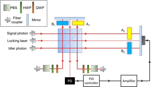
Figure A3. Experimental setup for implementing  entangled operation using a single UMI. This corresponds to the simplified version of the setup shown in figure A1. Note that the number of UMI is reduced from two to one, meaning that phase locking is required for only one interferometer.
Download figure:
Standard image High-resolution image
Figure A4. Experimental QST results with single UMI setup shown in figure A3. The realized entangled operation is  and the input state is
  . (a) ϕ = 4.15 and (b) ϕ = 4.80.
Download figure:
Standard image High-resolution imageTable A1. Comparison of experimental results obtained with the setups consisting of either single or double UMIs.
| 1 UMI | 2 UMIs | |
|---|---|---|
| Purity | 0.942 ± 0.018 | 0.904 ± 0.025 |
| Fidelity | 0.967 ± 0.010 | 0.940 ± 0.015 |
| Concurrence | 0.945 ± 0.017 | 0.906 ± 0.025 |
Appendix B.: Additional data of QST and QPT
In this section, we provide additional experimental data that are not included in the main text. At first, figure B1 shows the reconstructed output states after applying  entangled operation and the expected output state is
  for the input state
  . See figure 3 of the main text for comparison.

Figure B1. Reconstructed density matrices of the output state after the entangled operation  . Input state is prepared to |HV⟩ and the expected output state after the entangled operation is
  . The reconstructed density matrices of the output states correspond to (a) ϕ = 0, (b) π/2, (c) π, and (d) 3π/2. Note that the upper (lower) rows corresponds to the real (imaginary) part of the density matrices. The average fidelity between the ideal output state and the experimentally obtained output state is Fave = 0.933 ± 0.010 and the average concurrence of the output states C = 0.904 ± 0.018. We performed Monte-Carlo simulations on reconstructing density matrices of each output state 100 times and calculated experimental errors. Here the errors on each quantity corresponds to one standard deviation.
Download figure:
Standard image High-resolution imageFurthermore, we perform QPT measurement on  entangled operation and the experimentally reconstructed process matrix χexp is shown in supplementary figure B2. The process fidelity of χexp with respect to the ideal operation is 0.830 ± 0.008, which is obtained by performing Monte-Carlo simulations 100 times on the experimental data and the error corresponds to one standard deviation.

Figure B2. Experimentally reconstructed process matrices χ of the entangled operation  . Left (right) columns corresponds to the real (imaginary) part of the process matrices. Process matrices are represented in the Pauli basis.
Download figure:
Standard image High-resolution image